Chapter 2: Likelihood and Parameter Estimation/Fitting

When we have a theoretical prediction of a specific distribution, a model, we can estimate the parameters of the model given a experimental measurement. An example could be for example the exact value of the Higgs boson mass or the cross section of a particular final state or an angular distribution that may both depends on coupling structure/strength.

To get the best ‘fit’ of the model to the data we use a likelihood fit. It provides a measure of the (relative) compatibility of different parameter values of the model. With the metric we can determine both the central values of the model parameters that best describe the data together with the uncertainty on that number. Parameter estimation has been extensively covered in the lectures, here we just do the bare minimum required to make the exercises.

Binned likelihood

A likelihood refers to the compatibility of a set of model parameters with a specific data set.In our example we will define the (binned) likelihood by the product of the per-bin probabilties. In each bin we can use the Poisson distribution. The full likelihood is then given by:

\({\rm Likelihood} = \prod_{\rm bins} Poisson(n | {\rm model})\), which in use the

The goal is to find the set of model parameters that maximizes the likelihood.

Using the more practical -2Log(Likelihood)

With many bins, the likelihood is a very small number. To avoid numerical instabilities we always use minus twice the logarithm of the likelihood.

\({\rm -2 \cdot Log(Likelihood)} = -2\sum_{\rm bins} {\rm Log(Poisson(n | model))}\), which in use the

Maximizing the likelihood means minimizing the -2Log(Likelihood). For a model with one parameter this is ‘easy’ to do (and we will do this in the exercises), but it gets very complex very fast when multiple parameters are involved. There we rely on modelling and fittinhg frameworks like RooFit. One of the most famous ‘minimizers’ that we use in HEP is Minuit.

Extracting parameters: \(\Delta\)( -2Log(likelihood))

The ‘best’ value of the model parameters are the ones that minimize the -2Log(likelihood) distribution. Moving away from the optimal parameters will result in a worse value of the -2Log(likelihood). The one (two) sigma uncertainty is given by the value of the parameter that results in a value of -2Log(likelihood) that is one (four) different from the value in the minimum.

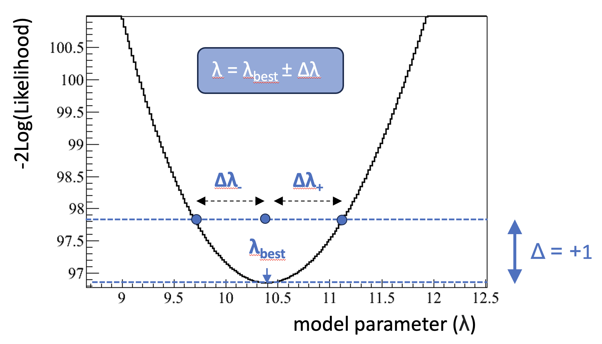
This last point is easy to understand if you see that if the likelihood follows a normal distribution, the -2Log(likelihood) distribution will be a parabola:

\(f(x) = e^{-\frac{1}{2}\left(\frac {x-\mu}{\sigma} \right)^2}\) \(\rightarrow [-2Log()] \rightarrow\) \(\left(\frac {x-\mu}{\sigma} \right)^2\)

Under the assumption of a parabola finding the minimizing is extremely simple for a minimizer, but for low statistics and more complex (correlated) models it is not that easy. In those cases the upper and lower uncertainty are not necessarily equal.

Use of likelihoods in the exercises

The likelihood depends of course on the model you evaluate. In the exercises 2 we will use the likelihood based on the background-only model to find a data-driven background estimate in the mass window by using the side-bands of the distribution. In exercise 3 we use the full model (SM + Higgs) model to find, simultaneously the background and Higgs boson cross-section scaling.

In part 3 we will use the ration of the likelihoods computed wither with of without the Higgs boson present to construct a variable that allows us to be more sensitive to a possible Higgs signal that the simple counting experiment we used in exercise 1.