Chapter 3: Test statistics and hypothesis testing

In this part of the analysis walkthrough we'll explore how to go beyond event counting from part 1 and to use the likelihood fits from section 2 to construct a variable that is more sensitive to differences between the two hypotheses: SM and SM + Higgs.

We will first define the variable (a single number – a test statistic) that we’ll use to indicate the compatibility with the two hypothese: the likelihood ratio X. We will then see how we can generate use toy-datasets to construct the distribution of X that we can then use to study how we can extract expected and observed significances and the exclusion limits for the signals.

Test statistic and ordering rule

In part 1 we have used the number of events to idicate if an experient is more background-like or more signal-like. There are more possibilities. Typically the difference between the signal and background processes is multi-dimensional and multivariate techniques (BDT's, transformers, neural networks) are used to condense an event into a single number and you can also do that for a full data-set. In our case we will define a new test statistic which based on the likelihood based on the two hypotheses.

\(X =-2 \cdot {\rm Log}(Q)\) with \(Q=\frac{L(s+b)} {L(b)}\)

with L(b) and L(s+b) the liklihood for the background-only and signal+background hypothesis respectively. In part 2 we saw that in a general way the likelihood for our model can be written as:

\({\rm -2 \cdot Log(Likelihood)} = -2\sum_{\rm bins i} {\rm Log(Poisson(n_{\rm bin}^{\rm evts} | \alpha \cdot f_{\rm SM} + \mu \cdot f_{\rm Higgs} ))}\)

If we look at the definition of X we end up with”

\(Q =\frac{L(\mu=1)} {L(\mu=0)}\)

Which leads to $ X = -2 \cdot {\rm Log}(L(\mu=1)) -2 \cdot {\rm Log}(L(\mu=0))$

Distribution of the test statistics

For a specific data-set the test-statistic is just a single number and to interpret its (in)compatibility with different hypotheses it is important to know the distribution for the test test statistic for data-sets that originate from the two hypotheses. This is similar in the case of event counting in exercise 1 where the Poisson distribution indicated the distribution of expected number of events for the SM and SM+Higgs hypotheses. Only when you have these distributions we can look at 'overlap' and make interpretations in terms of (in)compatibility.

Generation of Toy Data-Sets

To create the distributions of the test-srtatistic we can use so-called fake data-sets. These are data-sets that are created from the simulated template-histograms of the model and that reflect the expected statistical fluctuation.

Concretely:

• create an (empty) histogram identical to the one describing the model.
• Loop over the bins and in each bin: a) first get the number of events predicted by the model (\(\lambda_i\)) b) Draw a random number \(n_i\) from a Poisson distribution with that value as mean: Random->Poisson((\(\lambda_i\))).

Note that the number of events in each bin is random and look in the skeleton code on how to draw this random number in Root. If you do this for all bins you creat a fake data-set reflecting the random fluctuation that can occur in the measurement.

For each fake data-set you can compute the test statistic X and using a large number of these data-sets we can obtain the distribution of X. Note that these fake-dataset can be created under two assumptions: the model with the Higgs or the model with only the background.

Distribution of the test statistic and interpretation

A general example of the distribution for the likelihood ratio test statistic is shown in the plot. Note that being more background-like means moving towards the right. And reversely, moving towards the left is more signal like. It is good to remind yourself that the value of the test statistic in the data \(X_{\rm data}\) is of course only a single number.

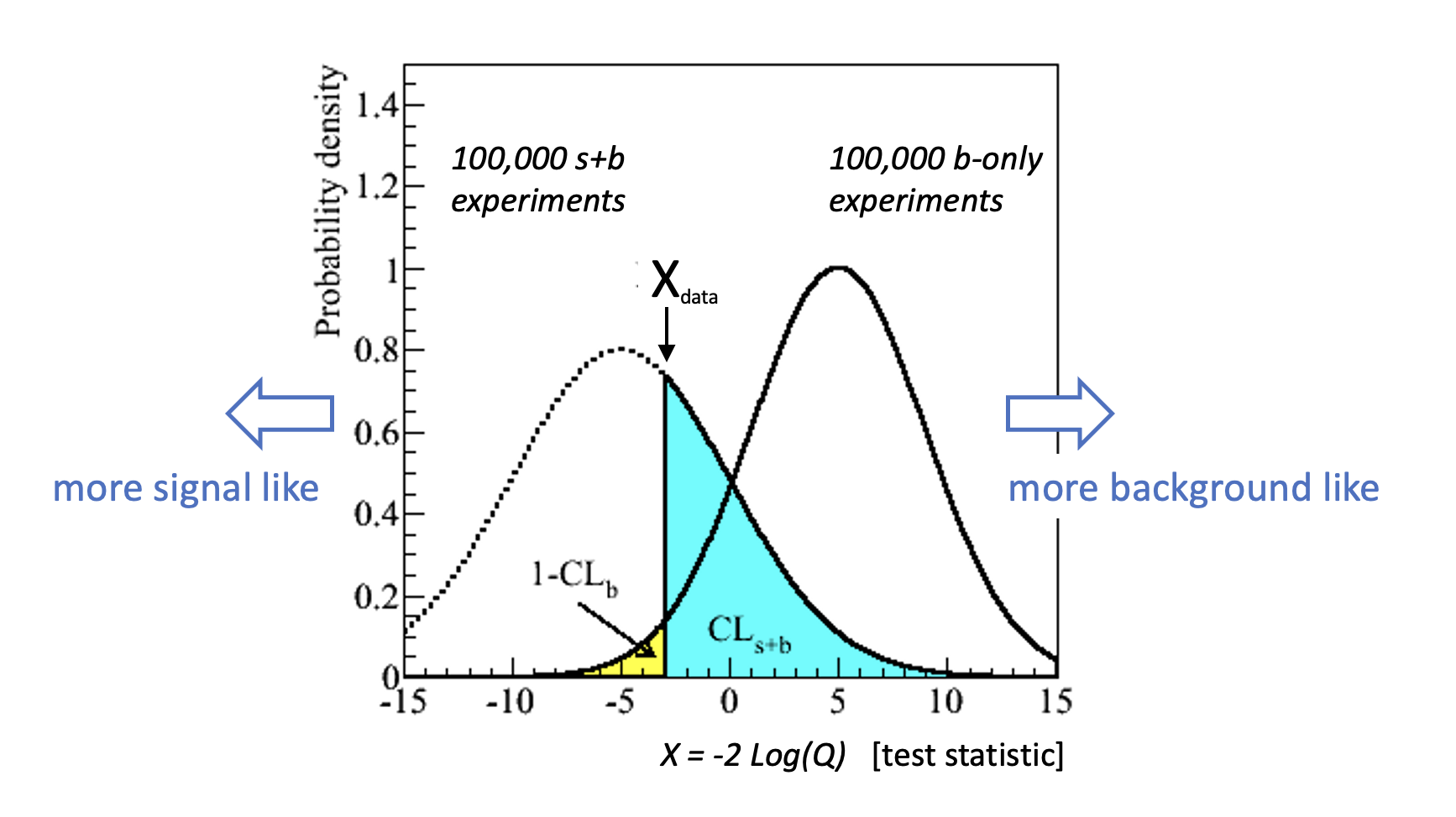
In a similar as was done in chapter 1 for the counting experiment we can define the (in)compatibilities with the two hypothesis. Although different names are used, we have seen these values before:

• For the compatibility with the backgorudn-only hypothesis, the 1-\(Cl_{b}\) (one minus the confidence level in the background) is the p-value we saw earlier as it indicates the probability to observe this value of the test statistic (or even more signal like) under the background hypothesis.

• For the compatibility with the signal+background hypothesis the \({\rm CL_{s+b}}\) (the confidence level in the signal + background) also looks familiar as that was the metric used to see if we could reject a new-physics hypothesis as it reflects the probability to observe this value of X (or even more background like) under the assumption of the signal+background hypothesis.

In a similar way to the counting experiment in chapter 1 we can define expected and observed p-values and (in)combatibilities with the various hypothesis. This allows us to answer similar questions related to expected and observed p-values and changes with increased data-sets and alternate Higgs production cross-sections. Exercises 4-7 will do just that.